This article covers light-source engineering and device parameters only. It does not evaluate clinical outcomes or define clinical indications, and the tissue-optics figures cited are public literature values that you should verify against your own tissue model and measurements. GK Semiconductor supplies light-source components; it does not provide medical advice and does not make regulatory, certification or laser-safety classification determinations. Those remain with the device builder under the regulations of the target market.
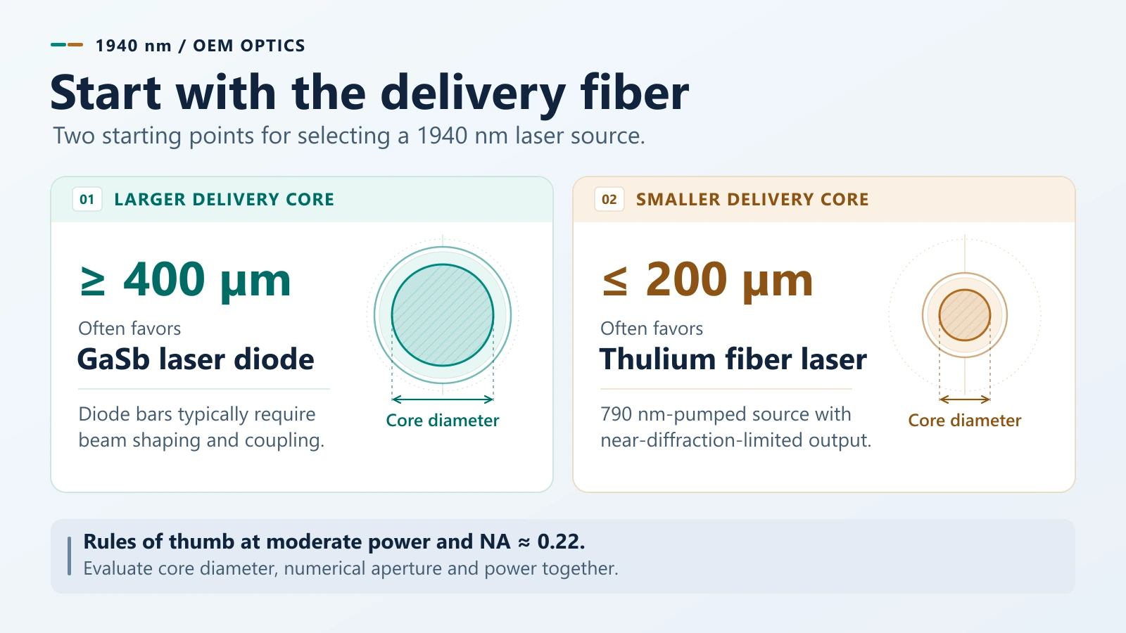
The short answer: choose a GaSb diode for a delivery fiber of ≥ 400 μm, and a thulium fiber laser for ≤ 200 μm. The conversion efficiencies of the two routes sit within the same order of magnitude and cannot be subtracted from one another; the diode's definite advantage is the missing pump stage, and the fiber laser's definite advantage is a near-diffraction-limited beam at the connector.
What Are the Key Takeaways?
l The physics. 1.94 μm sits on the O–H stretch-and-bend combination band, more than 100 nm wide. On public pure-water absorption data the coefficient is about 120 cm⁻¹, giving a 1/e absorption depth of about 0.08 mm in pure water; in soft tissue, scattering brings the effective thermal zone to the commonly quoted 0.1–0.2 mm. That is a literature figure, not a clinical specification.
l Two routes. 1.94 μm can come from a GaSb diode emitting directly, or from a 790 nm-pumped thulium-doped fiber. This article covers only those two. In-band pumping at 1.7/1.9 μm and cascaded pumping reach higher theoretical efficiency and would change the efficiency judgement; they are out of scope.
l How to compare efficiency. The diode figure is chip-level P_opt ÷ (I_op × V_op): 15.6–17.9 % for the single emitters and the 10 W bar, excluding driver, TEC and coolant pump. The fiber figure generally published is slope efficiency against absorbed pump power — a different boundary. A fair comparison means aligning every loss term; this article therefore gives no single cross-architecture number.
l Where the diode wins. Not conversion efficiency — chain length: no pump stage, one material system, direct electrical modulation, cm-scale packaging.
l Where the fiber laser wins. Not power — brightness: near-diffraction-limited output straight out of the fiber, with the whole free-space shaping chain removed.
l The boundary is not one threshold. The 400 μm and 200 μm figures must be read together with power and NA; quoting them alone leads to wrong architecture calls.
Selection at a glance
| Your constraint | Favour the diode | Favour thulium fiber |
| Delivery fiber core | ≥ 400 μm | ≤ 200 μm |
| Bend radius | Loose; rigid or semi-rigid applicator | Tight; through a working channel |
| Size and weight | Handheld, battery-powered, cm-scale package | Console with spool space |
| Drive | Gating / pulse shaping from the current | External modulation or AOM acceptable |
| Cost structure | BOM-sensitive, single material system | Second supply chain acceptable |
| Brightness headroom | Near-diffraction-limited output not needed | Near-diffraction-limited output required |
Which Questions Does This Article Answer?
1. Why is energy deposition at 1.94 μm concentrated in 0.1–0.2 mm?
2. How much optical power can a GaSb diode source deliver, and in what form factor?
3. How should the efficiencies of a diode and a thulium fiber laser be compared — and why can't they be subtracted?
4. Where does beam quality force an architecture decision?
5. What does 0.35 nm/°C of drift actually affect?
6. What should be settled before requesting a quote?
1. Why Is Energy Deposition at 1.94 μm Concentrated in 0.1–0.2 mm?
Because the wavelength sits on a strong water absorption band, and the light is largely gone within tens of micrometres.
Water absorbs at 1.94 μm because the wavelength falls on the combination band of the O–H stretch and bend — a band more than 100 nm wide, not a narrow line. That single fact governs everything later about drift and spectral width.
On public pure-water absorption data (derived figures, trend reference only):
| Wavelength | Absorption coefficient | 1/e depth in pure water |
| 980 nm | about 0.45 cm⁻¹ | about 22 mm |
| 1470 nm | about 25 cm⁻¹ | about 0.40 mm |
| 1940 nm | about 120 cm⁻¹ | about 0.08 mm |
| 2940 nm | about 1.27×10⁴ cm⁻¹ | about 0.8 μm |
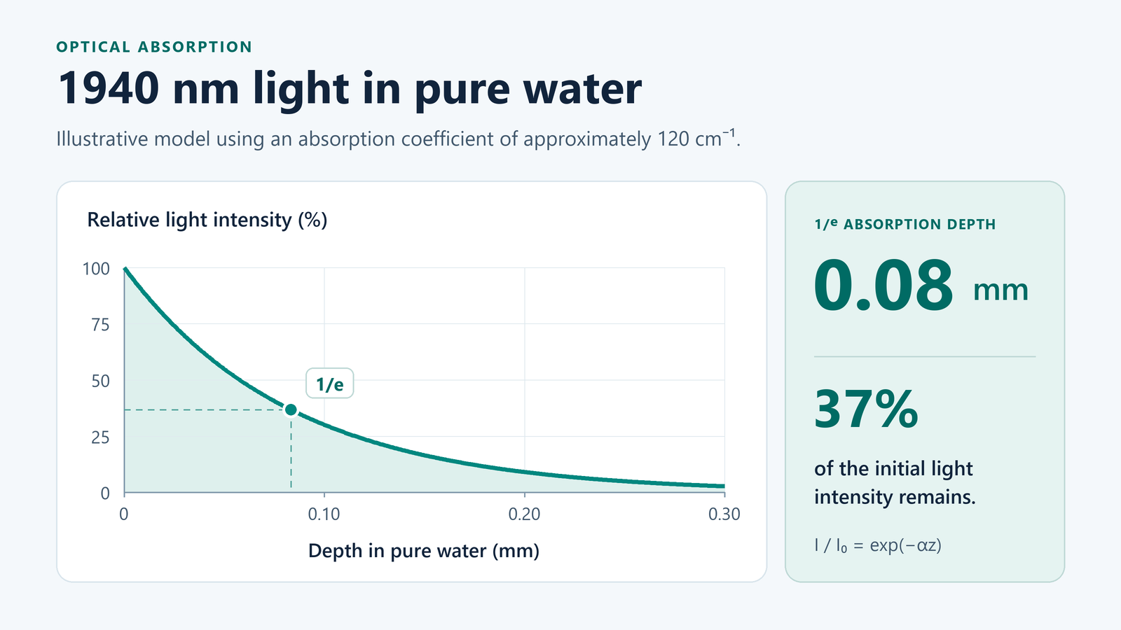 On that basis, 1.94 μm is absorbed roughly 266× more strongly than 980 nm (about 2.4 orders of magnitude) and 4.8× more strongly than 1470 nm; 2940 nm is another ~100× stronger again (the subject of the companion 2940 nm article, and the reason Er:YAG exists).
Two boundaries must be kept apart here, or the comparison goes wrong:
l 1/e absorption depth in pure water is an optical quantity set only by the absorption coefficient. At 980 nm it is 22 mm, centimetre scale. The 0.08 mm figure above belongs to this category.
l Effective penetration in tissue is set by absorption and scattering. At 980 nm it is only 1–3 mm in tissue, because scattering dominates; 1470 nm lies in between; 1940 nm is about 0.1–0.2 mm.
For 1940 nm the two boundaries are close — both sub-millimetre. For 980 nm they are far apart. Comparing 1940 nm's pure-water depth against 980 nm's tissue penetration overstates the gap.
What matters downstream is the geometry: energy deposited in a 0.2 mm shell can be confined to a target structure at a known depth. Fiber positioning tolerance, power setting, pull-back speed and cooling requirement all follow from that one number.
Three points need stating plainly:
l Absorption depth is a material property, not a clinical specification. It changes with water content and perfusion. Treat published values as design inputs, never as guarantees.
l Single-pass absorption depth is not the working depth of a finished system. Greater depth comes from repeated deposition, scanning and pull-back — an applicator and treatment-planning question. This article neither evaluates it nor sets application limits.
l Tissue is not pure water. Protein, lipid and blood content shift the measured absorption away from the pure-water value; calibrate that deviation against your own tissue model.
2. How Do Diodes and Thulium Fiber Lasers Both Reach 1940 nm?
The diode emits directly from epitaxy; the fiber converts pump light inside a doped core. One drops the pump stage, the other drops the beam-shaping chain.
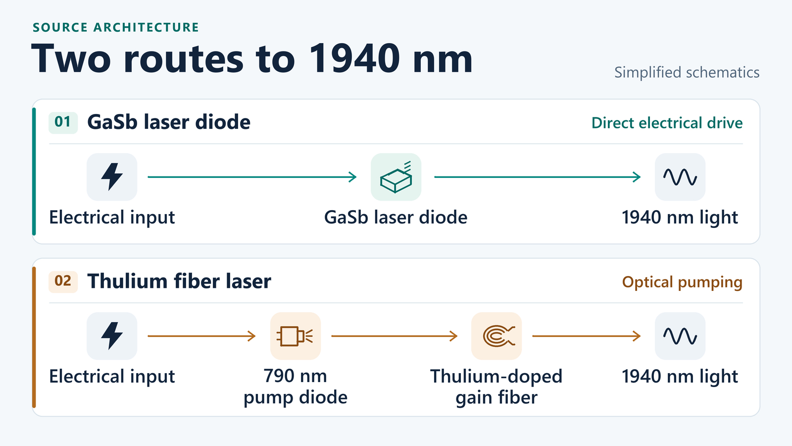
2.1 Can a GaSb Diode Emit at 1940 nm Directly?
Yes — no nonlinear conversion involved.
Antimonide emitters reach 1.94 μm by band-structure engineering on a GaSb substrate. GK Semiconductor grows, processes and packages these in-house, which matters mainly for one reason: wavelength and power are set at the epitaxial level, so a request for a slightly different centre wavelength is an epitaxy question, not a new laser architecture — though it is still an engineering evaluation, not a catalogue checkbox.
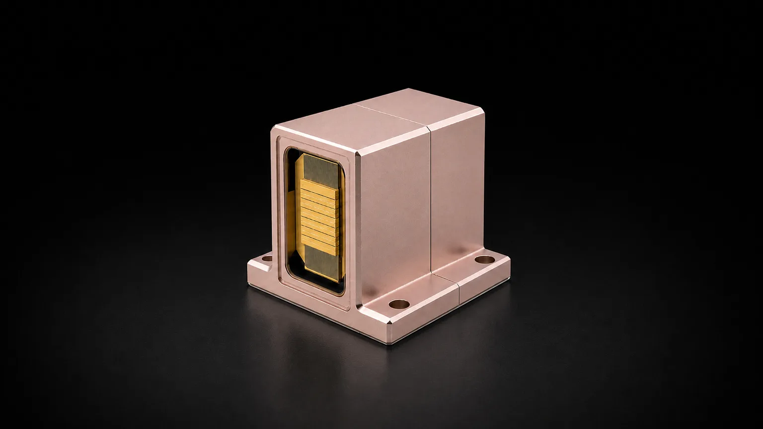
The catalogue spans three form factors:
| Form factor | Part number | Output | Emitter geometry | Typical use (application-dependent) |
| Single emitter | 1940-001W | 1 W CW | 150 μm stripe, 1000 μm cavity | Low-power OEM module |
| Single emitter | 1940-001.5W | 1.5 W CW | 200 μm stripe, 2000 μm cavity | Mid-power OEM module |
| Single emitter | 1940-002W | 2 W CW | 400 μm stripe, 2000 μm cavity | Module with relaxed brightness demand |
| Bar | GKBAR-1940-10W-CW-17 | 10 W CW | 19 emitters, 30 % fill factor, 500 μm pitch | Pumping, stack building block |
| Water-cooled stack | GKDZ-1940-050W-A7 | 50 W CW | 6 bars, 2.5 mm pitch; 4 L/min coolant flow, 25 °C recommended (15–35 °C) | Medical-aesthetic module (datasheet positioning) |
One clarification this band is frequently sloppy about: the 50 W module is a six-bar, water-cooled stack with free-space output, not a fiber-coupled module. If a specification sheet describes a 50 W 1.94 μm unit as "fiber coupled," ask for the fiber core diameter and the measured coupling efficiency. Fiber delivery at this power is a real engineering problem, not a line item. An output fiber, an articulated arm and a chiller can be supplied as matched accessories — a delivery add-on, not a fiber-coupled power specification. A coupled power figure is only issued once the coupling design is qualified against your fiber.
2.2 How Does a 790 nm-Pumped Thulium Fiber Laser Convert the Wavelength?
Pump light at 790 nm is coupled into a thulium-doped silica fiber, and Tm³⁺ converts it to 1.94 μm inside the core.
The output is near-diffraction-limited, circular, and already inside a fiber — for a system architect, that removes the entire free-space beam-shaping chain. This is the fiber route's most concrete benefit.
The cost is paid elsewhere:
l Quantum defect and cross-relaxation. 790 nm in, 1940 nm out: the single-ion Stokes ratio is 40.7 %, so if every ion worked alone, 59 % of the absorbed pump power would become heat. At the Tm³⁺ concentrations used in high-power fiber, cross-relaxation ("two-for-one") lets one excited ion hand energy to a ground-state neighbour, leaving both ions in the ³F₄ upper laser level: one pump photon produces two upper-level ions. Quantum efficiency in photon-count terms can therefore exceed 100 %; energy conservation still caps the energy-conversion efficiency at roughly 80 %. Public literature reports slope efficiencies in the 50–60 % range, depending on pump scheme and device design.
l Pump brightness and supply chain. The whole chain is only as good as the 790 nm pump diode — and that pump is GaAs-based, a different material system and a second supply chain from the GaSb emitter you would otherwise buy.
l Thermal load in the gain fiber. Heat is distributed along metres of fiber rather than concentrated in a 1 mm cavity — good for peak temperature, awkward for packaging.
Scope note: these conclusions apply to 790 nm pumping only. In-band pumping at 1.7/1.9 μm and cascaded pumping reach higher theoretical efficiency and would change the judgement in Section 3; they are out of scope here.
3. How Should the Efficiencies Be Compared?
You cannot subtract one from the other: the two sides are not measuring the same thing.
The diode figure is chip-level electro-optical conversion; the fiber figure generally published is slope efficiency against absorbed pump power. The loss terms in between decide what any "chain efficiency" number is really worth.
3.1 The Diode Side: Computable
Take P_opt ÷ (I_op × V_op) at datasheet operating points to get the chip-level conversion. This excludes driver loss, TEC and coolant pump, and also excludes beam shaping and fiber coupling. Add threshold current and slope efficiency becomes independently checkable.
| Source | Operating point | I_th | Electrical input | Optical output | Chip-level wall-plug | Slope efficiency |
| 1940-001W | 3.5 A @ 1.7 V | 0.3 A | 5.95 W | 1 W | 16.8 % | 0.31 W/A |
| 1940-001.5W | 6 A @ 1.4 V | 0.5 A | 8.4 W | 1.5 W | 17.9 % | 0.28 W/A |
| 1940-002W | 8 A @ 1.6 V | 1 A | 12.8 W | 2 W | 15.6 % | 0.28 W/A |
| GKBAR-1940-10W-CW-17 | 45 A @ 1.4 V | 5 A | 63 W | 10 W | 15.9 % | 0.25 W/A |
| GKDZ-1940-050W-A7 | at the model's rated operating point | — | per formal datasheet | 50 W | per formal datasheet | per formal datasheet |
(Check: wall-plug = P_opt ÷ (I_op × V_op); P_opt ÷ (I_op − I_th) reproduces the datasheet slope-efficiency figures to within rounding. Neither includes TEC, coolant pump or driver. Module-level electrical and conversion figures are issued with the formal datasheet and internal documents; no specific values are given here.)
3.2 The Fiber Side: Not Computable the Same Way
The 50–60 % commonly quoted for thulium fiber is slope efficiency against absorbed pump power, not absolute electrical-to-optical conversion. From pump electrical input to 1.94 μm output, at least six terms intervene: pump electro-optical conversion (and whether the driver is included is a separate boundary), pump combining loss, pump-to-fiber coupling loss, pump absorption (unabsorbed pump becomes heat), FBG and output-coupling loss, and threshold power.
Unless all six are stated, multiplying "pump electro-optical efficiency" by "slope efficiency" produces a number that is not on the same boundary as the diode's chip-level P/(I×V). It has not paid the losses, it has not counted the driver, and it is neither reproducible nor a sound basis for a conclusion. This article gives no such number; where one is needed, it should come from each side's formal datasheet and measurement report.
3.3 So the Comparison Lands on Chain Length, Not on an Efficiency Gap
This is boundary discipline, not evasion. Three statements can be made responsibly:
1. The two routes are within the same order of magnitude on wall-plug — not an order of magnitude apart.
2. Thulium fiber is not necessarily behind at high power; with a well-chosen pump scheme it can be better.
3. The diode's definite advantage is chain length — see below.
l No pump stage. No 790 nm pump diodes, no pump combiners, no doped fiber, no fiber Bragg gratings, no isolators. One fewer BOM segment, one fewer family of failure modes.
l One material system. GaSb epitaxy, chip and package in one chain — no second III-V supply chain.
l Direct electrical modulation. Gating and pulse shaping come from the drive current; a fiber laser needs external modulation or an acousto-optic element.
l Package scale. A centimetre-scale stack versus a fiber laser engine that needs spool space.
Whether 15–18 % is an advantage depends on what you compare it against and what you optimise for. In a battery-powered or fan-cooled handheld, size, weight, cost and instant-on matter more than a few points of wall-plug. In a mains-powered clinic console with a chiller already on the cart, wall-plug is a rounding error and brightness is the main term.
4. Where Does Beam Quality Force an Architecture Decision?
At the point you fix the delivery fiber core diameter — usually earlier than power or efficiency settles the architecture.
A diode bar is a line of 19 emitters, each with a fast axis diverging at tens of degrees. To get that into a 400 μm fiber you need fast-axis collimation, slow-axis collimation and a beam transformer — and you still pay a brightness penalty, because the emitters are spatially incoherent with one another. This is ordinary, well-understood optical engineering, but it is engineering you have to do, qualify and keep aligned through a thermal cycle.
A thulium fiber laser hands you near-diffraction-limited output at the connector (M² ≈ 1 is the ideal figure; use the datasheet value for the actual part). That is why fiber lasers dominate applications where the delivery fiber is small, bent repeatedly, or aimed through a working channel.
The boundary is not a single threshold. The 400 μm and 200 μm figures assume a typical 0.22 NA and moderate power; as power rises, NA falls and core diameter shrinks, the diode route's shaping difficulty and losses rise with them. Read the three together — the selection table sits at the top of this article.
5. What Does 0.35 nm/°C of Drift Actually Affect?
Very little, as far as absorption goes. The real reasons for temperature control are specification and batch consistency.
The GK 1940 nm diode family drifts at 0.35 nm/°C. Across the specified 15–35 °C operating range, that is 7 nm of centre-wavelength movement.
At this magnitude, absorption barely moves. 1.92–1.94 μm sits on the inner slope of a broad absorption band, and public measurements show the water absorption coefficient changing by only single-digit percent (about 5 % order) across that span, which moves the 1/e depth by less than 10 %. You do not need temperature control in order to "sit on a water absorption line" — water is broadband here.
So is temperature control still needed? Yes, for three other reasons:
1. Specification consistency. The part is specified at 25 °C; a system running in a 15–35 °C environment will see its wavelength move by 7 nm. If your coatings, filters and fiber passbands are designed around the nominal wavelength, that tolerance belongs in your requirements.
2. Batch and unit-to-unit consistency. Multiple systems and multiple lots need reproducible output; temperature control is the cheapest way to get there.
3. Staying off the system edges. Coating bands, fiber transmission windows and detector response edges all have boundaries. 7 nm is not frightening in itself; crossing an edge is.
This is not a defect — it is what a Fabry–Perot diode does. But it is the kind of item discovered at integration, after the mechanical envelope is frozen. Put it on the requirements list in week one.
On spectral width: the 10 W bar is specified at 8 nm, the single emitters at 13 nm, and the 50 W module at 13 nm. The measurement definition and the bar screening rule are set by the formal datasheet and internal documents — figures taken under different definitions are not comparable, and "is 7 nm more than half the spectral width" is not a sound way to judge engineering impact.
6. What Should Be Settled Before Requesting a Quote?
Ten items. The first one usually decides the architecture on its own.
1. Delivery geometry. Fiber core diameter, numerical aperture, bend radius, connector type. This single answer usually decides the architecture.
2. Required power at the tissue, not at the source. Coupling and fiber losses are yours to model; ask for the source-referenced number and do the rest yourself.
3. Duty cycle and thermal path. CW at 50 W into a small applicator is a heat-transfer problem before it is an optical one. Specify coolant flow, inlet temperature and allowable case temperature.
4. Wavelength tolerance and control. Centre wavelength, tolerance band, and whether the TEC sits inside your enclosure or ours; TEC power draw belongs in the system budget.
5. Pulse and gating format, if any. The 1.94 μm diode family is specified CW. If you need gated operation, say so early — beyond a different driver design, you need to specify peak current, duty cycle and derating, and their effect on lifetime. Exact gating specifications are issued with internal documents and engineering response.
6. Volume and lifetime target. Diode degradation is gradual and measurable; fiber-laser failure modes such as photodarkening or transverse mode instability can appear more abruptly. The reliability question you should ask differs by architecture.
7. Laser safety and protection requirements. Target classification, interlock scheme, fiber-break detection method (see next section). This decides whether the source side needs monitoring interfaces at all.
8. Measurement and acceptance conditions. Power-meter calibration, steady-state criterion (how long until "stable"), ambient temperature, spectral-width definition. Without these, factory numbers will not match your bench numbers.
9. Driver and control boundary. Constant current or constant power, soft-start ramp, over-current and over-temperature thresholds, whether an external modulation interface is needed.
10. Change control and datasheet revision. Lock one datasheet revision as the acceptance basis; any later parameter change goes through a written change notice, so lots cannot drift quietly.
Laser Safety and Compliance Boundaries at Integration
The division is clear: GK owns the source-side parameters; the integrator owns system-side classification, protection and registration.
1940 nm at 50 W CW falls in the Class 4 power range under the IEC 60825-1 / GB 7247.1 classification system. The actual classification, labelling and protection design are determined and owned by the device builder for the final configuration — GK supplies a light-source component, not a finished system, and makes no certification or registration determination. Which regulatory category the finished device falls into, and which registration route it takes, is decided under the target market's current rules; GK does not answer that on the customer's behalf.
At least these items belong in the integration plan:
l Protective interlocks. Applicator, enclosure and fiber connector states must be able to cut the emission.
l Fiber break and core-break detection. 1.94 μm is invisible; a broken fiber gives the operator no visual warning, so back-reflection or scatter monitoring is required.
l Back-reflection isolation. Light reflected from tissue or a workpiece disturbs a Fabry–Perot diode and can damage the facet at high power; the thulium fiber route needs an isolator for the same reason.
l Coolant flow-loss and condensation protection. 25 °C coolant condenses in humid environments; flow loss must interlock, and a minimum flow must be enforced. Exact water-loop boundaries (pressure, water quality, dew-point margin) follow the formal datasheet and the system design.
l Electrical safety. If the system is designed to IEC 60601-1 / -2-22, the source supply, isolation and leakage current belong in that assessment.
This section is not a disclaimer — it is a division of responsibility. Raising the first four items during the specification conversation is far cheaper than changing the design afterwards.
FAQ: What Do OEMs Ask Most About 1940 nm Sources?
Is a 1940 nm diode more efficient than a thulium fiber laser?
You cannot compare them with a single number. The diode figure is chip-level P_opt ÷ (I_op × V_op), 15.6–17.9 %, excluding driver, TEC and coolant pump; the fiber figure usually published is slope efficiency against absorbed pump power, commonly 50–60 % — a different boundary. A fair comparison has to align threshold, combining and coupling losses, pump absorption, FBG and output coupling, and the driver — and that requires measured data on both sides. What can be said: they are in the same order of magnitude, and thulium fiber is not necessarily behind at high power. The diode's definite advantage is the missing pump stage: BOM, package size, direct modulation, one material platform.
Can I get 50 W out of a fiber?
Not from the GK 50 W module, which is a six-bar free-space stack. Fiber delivery at that power requires a coupling design evaluated against your fiber, not assumed from a power number. An output fiber, an articulated arm and a chiller can be supplied as matched accessories — but a fiber-coupled power figure is only issued once the coupling design is qualified.
Does 7 nm of drift change the absorption much?
No. 1.94 μm is a broadband absorber; 7 nm changes the absorption coefficient by single-digit percent and the 1/e depth by less than 10 %. Temperature control is still worthwhile, but for specification consistency, batch consistency and staying off system edges — not for "locking to an absorption line."
Do I need a chiller for the 50 W module?
Yes — plan the coolant loop before the optical bench: 4 L/min at a recommended 25 °C operating temperature (15–35 °C range). The pressure drop is set by your own loop design; we do not publish a separate pressure limit outside the datasheet. Flow-loss interlocks and dew-point protection belong on the system side. Detailed water-loop boundaries follow the formal datasheet.
Can GK supply the fiber-coupled version?
Coupling schemes for the single-emitter parts are an engineering discussion, and we will quote what we can measure. We will not put a fiber-coupled power figure on a 50 W stack until the coupling design is qualified against your fiber.
Next Step: How Do You Get Measured Data and Samples?
Start with a specification conversation, not a catalogue download.
We build 1.94 μm sources from GaSb epitaxy through packaged module, so wavelength, emitter geometry and package can be set together rather than sourced separately. For device builders evaluating this band, the useful next step is to put delivery geometry, power budget and thermal path on the table.
l Request Datasheet & Test Report — measured L-I-V, spectrum and thermal data for the part you are considering.
l Inquire for Engineering Sample — single emitters and bars available for bench evaluation.
Related: How to spec a light source for medical aesthetic lasers · 2940 nm Er:YAG for OEM systems · 808 nm QCW bars
Product pages: 1940 nm 50 W module · 1940 nm 10 W bar · 1940 nm 2 W · 1940 nm 1.5 W